Recurrent Neural Net From Scratch¶

I will skip the reasoning behind why we need RNN. There's plenty on the internet. I'll focus on learning the technical side, and hope that the answers to "why"s will come naturally. This is the same principal as other notebooks in my "from scratch" series. This is heavily based on the basic neural net, so read that one first.

Recall that in a neural network, we have:

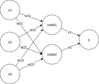
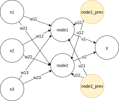
For recurrent neural network, we carry over info from the previous data point in the sequence, by incorporating the values of the hidden layer, with its own weight $u$.

Feed forward¶

Rephrasing the diagram, we have the feed forward process as, for each time step $t$,

• $s_{h,t} = x_t W + a_{h,t-1}U + b_h$
• $a_{h,t} = \sigma_h(s_{h,t})$
• $s_{o,t} = a_{h,t}V +b_o$
• $y_t = \sigma_o(s_{o,t})$

h means hidden layer, o means output layer, s means weighted sum, a means activated value. $\sigma$ means the activation function. For the activation functions, we use softmax at the output layer and tanh at the hidden layer.

$$\large tanh(x) = \frac{e^x - e^{-x}}{e^x + e^{-x}} $$

It has the convenient property that

$$ \large (tanh(x))' = 1-(tanh(x))^2 $$

Backpropagation Through Time¶

• As there's dependency bewteen the previous and next steps, backpropagation in RNN goes through the entire sequence, called Backpropagation Through Time (BPTT) where we propagate the gradient not only through layers, but also through the entire sequence of data. This means we sum up the lost of the predictions of the sequece.

Overall loss is

$$ L_{total} = \sum_1^t L_t $$

where

$$ L_t = -y_t log(\hat{y_t}) $$

• Backpropagation from the output layer to the hidden layer is similar as vanila neural network since we don't add anything new between these two layers
• Backpropagation from the hidden layer will go to both the input layer and the hidden layer of the previous data point.

Weights from the output layer to the hidden layer¶

From the math of basic neural net, we know

$$ \large \frac{\partial L_t}{\partial V} = (\hat{y_t} - y_t) \cdot a_{h,t} $$

Replace $a_h$ with 1 for the bias term

Weights from the hidden to the input layer and previous data point¶

From above setup, we can see that $s_{h,t}$ is an important term as it's a function of $W, U, a_{h,t-1}$. In backpropagation, the gradient will flow from $s_{h,t}$ to those components like the following, based on the formula in the feedforward section above:

$$\large \begin{align} \frac{\partial L_t}{\partial W} &= \frac{\partial L_t}{\partial s_{h,t}} \cdot x_t \\ \frac{\partial L_t}{\partial U} &= \frac{\partial L_t}{\partial s_{h,t}} \cdot a_{h,t-1} \\ \frac{\partial L_t}{\partial b_h} &= \frac{\partial L_t}{\partial s_{h,t}} \end{align} $$

To get $\Large \frac{\partial L_t}{\partial s_{h,t}}$, we have

$$\large \begin{align} \frac{\partial L_t}{\partial s_{h,t}} & = \frac{\partial L_t}{\partial a_{h,t}}\cdot \frac{\partial a_{h,t}}{\partial s_{h,t}} \\ & = \frac{\partial L_t}{\partial a_{h,t}}\cdot \frac{\partial \sigma_h(s_{h,t})}{\partial s_{h,t}} \\ & = \frac{\partial L_t}{\partial a_{h,t}}\cdot (1-(tanh(s_{h,t}))^2) \end{align} $$

All we have left to derive is $\Large \frac{\partial L_t}{\partial a_{h,t}}$. As $\large a_{h,t}$ contributes to $L_{t+1}$, the gradient from $L_{t+1}$ also goes to $\large a_{h,t}$. Therefore

$$\large \begin{align} \frac{\partial L_t}{\partial a_{h,t}} &= \frac{\partial L_t}{\partial s_{o,t}} \cdot \frac{\partial s_{o,t}}{\partial a_{h,t}} + \frac{\partial L_{t+1}}{\partial s_{h,t+1}} \cdot \frac{\partial s_{h,t+1}}{\partial a_{h,t}} \\ &= (\hat{y_t} - y_t)\cdot V + \frac{\partial L_{t+1}}{\partial s_{h,t+1}} \cdot U \end{align} $$

Problem to solve¶

We'll use RNN to solve a toy problem of predicting the next number in mod 3. 1 is next to 0, 2 is next to 1, 0 is next to 2.

In [1]:

import numpy as np

# length of the sequence is the length of the problem. Keep it not too big for calculation, but not too small to be boring.
length = 50

x_num = [np.random.randint(0, 3) for i in range(length)]
y_num = [(x+1) % 3 for x in x_num]
x_str = ''.join([str(i) for i in x_num])
y_str = ''.join([str(i) for i in y_num])
print('input: ', x_str)
print('output:', y_str)

import numpy as np # length of the sequence is the length of the problem. Keep it not too big for calculation, but not too small to be boring. length = 50 x_num = [np.random.randint(0, 3) for i in range(length)] y_num = [(x+1) % 3 for x in x_num] x_str = ''.join([str(i) for i in x_num]) y_str = ''.join([str(i) for i in y_num]) print('input: ', x_str) print('output:', y_str)

input:  11220020221211221211112201122011202120001210122112
output: 22001101002022002022220012200122010201112021200220

Repeat to make a dataset

In [2]:

def num_to_label(y, vocab=3):
    # turn a single digit label to multiclass labels
    labels = np.zeros((len(y), vocab), dtype=int)
    for i, yy in enumerate(y):
        labels[i, yy] = 1
    return labels

def make_pairs(length=10, vocab=3):
    x_num = [np.random.randint(0, vocab) for i in range(length)]
    y_num = [(x+1) % vocab for x in x_num]
    # One hot encode the input and output
    x = num_to_label(x_num)
    y = num_to_label(y_num)
    return x, y

def num_to_label(y, vocab=3): # turn a single digit label to multiclass labels labels = np.zeros((len(y), vocab), dtype=int) for i, yy in enumerate(y): labels[i, yy] = 1 return labels def make_pairs(length=10, vocab=3): x_num = [np.random.randint(0, vocab) for i in range(length)] y_num = [(x+1) % vocab for x in x_num] # One hot encode the input and output x = num_to_label(x_num) y = num_to_label(y_num) return x, y

In [3]:

size = 10
x, y = [], []
for i in range(size):
    xx, yy = make_pairs()
    x.append(xx)
    y.append(yy)

size = 10 x, y = [], [] for i in range(size): xx, yy = make_pairs() x.append(xx) y.append(yy)

Different from basic neural net, RNN does feed forward and backpropagation for the entire sequence, not at each step independently. First let's layout the components we need. This should give a rough breakdown to help writing the code.

In [4]:

class RNN():
    def __init__(self):
        # initialize a random set of weigths and biases
        pass

    def predict(self):
        # this is the feed forward process
        pass

    def backpropagation(self):
        # one round of backpropagation through the entire sequence
        pass

    def train(self, epochs):
        pass

    def total_loss(self):
        pass

    def loss(self, t):
        return 

    def tanh(x):
        pass

    def softmax(x):
        pass

class RNN(): def __init__(self): # initialize a random set of weigths and biases pass def predict(self): # this is the feed forward process pass def backpropagation(self): # one round of backpropagation through the entire sequence pass def train(self, epochs): pass def total_loss(self): pass def loss(self, t): return def tanh(x): pass def softmax(x): pass

Then fill in the blanks. We'll first enable feed forward functions. In the init function, we not only need to initialize the parameters, but also reserve vectors to memorize all the calculations, as we'll rely on them in both feed forward and BTT. As we see above, terms like $\Large \frac{\partial L_t}{\partial s_{h,t}}$ are used multiple times and in different epochs.

In [31]:

import numpy as np

class RNN1():
    def __init__(self, n_nodes=10, vocab_size=3):
        # initialize a random set of weigths and biases
        self.n_nodes = n_nodes
        self.w = np.random.randn(n_nodes, vocab_size)
        self.u = np.random.randn(n_nodes, n_nodes)
        self.v = np.random.randn(vocab_size,n_nodes)
        self.b_h = np.random.randn(n_nodes)
        self.b_o = np.random.randn(vocab_size)
        self.s_h = []
        self.a_h = []
        self.s_o = []
        self.y_hat = []

    def predict(self, x):
        return [self.predict_single(xx) for xx in x]

    def predict_scores(self, x):
        return [self.feedforward(xx) for xx in x]
    
    def predict_single(self, x):
        scores = self.feedforward(x)
        return self.score_to_num(scores)

    def reset_mem(self):
        self.s_h = []
        self.a_h = []
        self.s_o = []
        self.y_hat = []
    
    def feedforward(self, x):
        self.reset_mem()
        # this is the feed forward process
        for t in range(len(x)):
            # this follows straight from the formula
            a_ht_prev = np.zeros(self.n_nodes) if t == 0 else self.a_h[t-1]
            s_ht = x[t] @ self.w.T + a_ht_prev @ self.u + self.b_h
            a_ht = self.tanh(s_ht)
            s_ot = a_ht @ self.v.T + self.b_o
            y_t = self.softmax(s_ot)

            # memorize all above
            self.s_h.append(s_ht)
            self.a_h.append(a_ht)
            self.s_o.append(s_ot)
            self.y_hat.append(y_t)
        return self.y_hat

    def total_loss(self, y, y_hat):
        return sum([self.loss(t, y, y_hat) for t in range(len(y))])

    @staticmethod
    def loss(t, y, y_hat):
        if (y[t] == y_hat[t]).all():
            return 0
        return np.sum(-y[t]*np.log(y_hat[t]))

    @staticmethod
    def tanh(x):
        return np.tanh(x)

    @staticmethod
    def softmax(x):
        x = np.array(x, dtype=np.float128)
        # to avoid overflow due to super large x, we subtract the max
        xx = x - np.max(x)
        exp = np.exp(xx)
        return exp / exp.sum(keepdims=True)

    @staticmethod
    def score_to_num(scores):
        indices = [np.argmax(p) for p in scores]
        return np.array(indices)

import numpy as np class RNN1(): def __init__(self, n_nodes=10, vocab_size=3): # initialize a random set of weigths and biases self.n_nodes = n_nodes self.w = np.random.randn(n_nodes, vocab_size) self.u = np.random.randn(n_nodes, n_nodes) self.v = np.random.randn(vocab_size,n_nodes) self.b_h = np.random.randn(n_nodes) self.b_o = np.random.randn(vocab_size) self.s_h = [] self.a_h = [] self.s_o = [] self.y_hat = [] def predict(self, x): return [self.predict_single(xx) for xx in x] def predict_scores(self, x): return [self.feedforward(xx) for xx in x] def predict_single(self, x): scores = self.feedforward(x) return self.score_to_num(scores) def reset_mem(self): self.s_h = [] self.a_h = [] self.s_o = [] self.y_hat = [] def feedforward(self, x): self.reset_mem() # this is the feed forward process for t in range(len(x)): # this follows straight from the formula a_ht_prev = np.zeros(self.n_nodes) if t == 0 else self.a_h[t-1] s_ht = x[t] @ self.w.T + a_ht_prev @ self.u + self.b_h a_ht = self.tanh(s_ht) s_ot = a_ht @ self.v.T + self.b_o y_t = self.softmax(s_ot) # memorize all above self.s_h.append(s_ht) self.a_h.append(a_ht) self.s_o.append(s_ot) self.y_hat.append(y_t) return self.y_hat def total_loss(self, y, y_hat): return sum([self.loss(t, y, y_hat) for t in range(len(y))]) @staticmethod def loss(t, y, y_hat): if (y[t] == y_hat[t]).all(): return 0 return np.sum(-y[t]*np.log(y_hat[t])) @staticmethod def tanh(x): return np.tanh(x) @staticmethod def softmax(x): x = np.array(x, dtype=np.float128) # to avoid overflow due to super large x, we subtract the max xx = x - np.max(x) exp = np.exp(xx) return exp / exp.sum(keepdims=True) @staticmethod def score_to_num(scores): indices = [np.argmax(p) for p in scores] return np.array(indices)

Run some random numbers to make sure matrix dimensions are good. We have written functions to

• Make predictinos by feed forward, using randomly generated parameters
• Calculate loss

In [32]:

rnn1 = RNN1()
pred_scores = rnn1.predict_scores(x)
pred = rnn1.predict(x)
loss = rnn1.total_loss(y, pred_scores)

rnn1 = RNN1() pred_scores = rnn1.predict_scores(x) pred = rnn1.predict(x) loss = rnn1.total_loss(y, pred_scores)

In [13]:

pred, loss, 

pred, loss,

Out[13]:

([array([1, 0, 0, 0, 1, 0, 0, 1, 1, 0]),
  array([2, 0, 0, 0, 1, 0, 0, 1, 2, 0]),
  array([1, 0, 2, 1, 0, 0, 2, 0, 0, 0]),
  array([1, 0, 2, 1, 0, 0, 0, 0, 1, 0]),
  array([1, 0, 0, 0, 1, 2, 2, 2, 0, 0]),
  array([2, 0, 0, 0, 0, 1, 0, 0, 1, 1]),
  array([1, 0, 2, 2, 0, 0, 1, 0, 1, 2]),
  array([2, 0, 0, 0, 1, 0, 0, 1, 1, 0]),
  array([2, 0, 0, 0, 0, 0, 1, 0, 0, 2]),
  array([1, 0, 0, 0, 1, 0, 0, 1, 1, 0])],
 np.longdouble('164.06705644911090597'))

In [10]:

# validate correctness of the loss calculation
loss0 = rnn1.total_loss(y[0], y[0])
loss1 = rnn1.total_loss(pred_scores[0], pred_scores[0])
assert loss0 == 0
assert loss1 == 0

# validate correctness of the loss calculation loss0 = rnn1.total_loss(y[0], y[0]) loss1 = rnn1.total_loss(pred_scores[0], pred_scores[0]) assert loss0 == 0 assert loss1 == 0

Move ahead to BPTT!

In [191]:

class RNN2(RNN1):
    def __init__(self, learning_rate=0.0001, n_nodes=10, vocab_size=3):
        super().__init__()
        self.learning_rate = learning_rate
        self.delta_l_over_s_h = []

    def backpropagation(self, x, y, y_hat):
        # BPTT for a single sequence of sample. This function
        # returns the deltas of W, V, U, b_h, and b_o
        T = len(y)
        du = np.zeros(self.u.shape)
        dv = np.zeros(self.v.shape)
        dw = np.zeros(self.w.shape)
        dbh = np.zeros(self.b_h.shape)
        dbo = np.zeros(self.b_o.shape)
        # btt goes backwards, from time t to time 0
        ds_ht_plus_1 = np.zeros(self.n_nodes)
        for t in reversed(range(T)):
            # one round of backpropagation at time t
            # output layer to hidden layer.
            # dLt/dbo = (y_hat_t - y_t)
            # dLt/dV = (y_hat_t - y_t) * a_ht = dLt/dbo * a_ht
            dbo_t = (y_hat[t] - y[t].T)
            dv_t = dbo_t[:, np.newaxis] @ self.a_h[t][:, np.newaxis].T
            dbo += dbo_t
            dv += dv_t

            # hidden layer to input layer
            da_ht = (y_hat[t] - y[t]) @ self.v + ds_ht_plus_1 @ self.u
            ds_ht = da_ht * (1-self.a_h[t] ** 2)
            ds_ht_plus_1 = ds_ht
            dw_t = ds_ht[:, np.newaxis] @ x[t][:, np.newaxis].T

            if t-1 >= 0:
                a_ht_1 = self.a_h[t-1]
            else:
                a_ht_1 = np.zeros(self.n_nodes)
            du_t = ds_ht @ a_ht_1

            dbh_t = ds_ht

            dw += dw_t
            du += du_t
            dbh += dbh_t
            
        return dw, dv, du, dbh, dbo

    def train(self, epochs, x, y, verbose=False):
        for i in range(epochs):
            loss = 0
            for j in range(len(x)):
                # feed forward
                y_hat = self.feedforward(x[j])
                # current loss
                loss += self.total_loss(y[j], y_hat)
                # calculate deltas
                dW, dV, dU, dbh, dbo = self.backpropagation(x[j], y[j], y_hat)
                # update weights accordingly
                self.u -= self.learning_rate * dU
                self.w -= self.learning_rate * dW
                self.v -= self.learning_rate * dV
                self.b_h -= self.learning_rate * dbh
                self.b_o -= self.learning_rate * dbo
            if verbose and i % 100 == 0:
                print(f"loss at epoch {i}: {loss}")

class RNN2(RNN1): def __init__(self, learning_rate=0.0001, n_nodes=10, vocab_size=3): super().__init__() self.learning_rate = learning_rate self.delta_l_over_s_h = [] def backpropagation(self, x, y, y_hat): # BPTT for a single sequence of sample. This function # returns the deltas of W, V, U, b_h, and b_o T = len(y) du = np.zeros(self.u.shape) dv = np.zeros(self.v.shape) dw = np.zeros(self.w.shape) dbh = np.zeros(self.b_h.shape) dbo = np.zeros(self.b_o.shape) # btt goes backwards, from time t to time 0 ds_ht_plus_1 = np.zeros(self.n_nodes) for t in reversed(range(T)): # one round of backpropagation at time t # output layer to hidden layer. # dLt/dbo = (y_hat_t - y_t) # dLt/dV = (y_hat_t - y_t) * a_ht = dLt/dbo * a_ht dbo_t = (y_hat[t] - y[t].T) dv_t = dbo_t[:, np.newaxis] @ self.a_h[t][:, np.newaxis].T dbo += dbo_t dv += dv_t # hidden layer to input layer da_ht = (y_hat[t] - y[t]) @ self.v + ds_ht_plus_1 @ self.u ds_ht = da_ht * (1-self.a_h[t] ** 2) ds_ht_plus_1 = ds_ht dw_t = ds_ht[:, np.newaxis] @ x[t][:, np.newaxis].T if t-1 >= 0: a_ht_1 = self.a_h[t-1] else: a_ht_1 = np.zeros(self.n_nodes) du_t = ds_ht @ a_ht_1 dbh_t = ds_ht dw += dw_t du += du_t dbh += dbh_t return dw, dv, du, dbh, dbo def train(self, epochs, x, y, verbose=False): for i in range(epochs): loss = 0 for j in range(len(x)): # feed forward y_hat = self.feedforward(x[j]) # current loss loss += self.total_loss(y[j], y_hat) # calculate deltas dW, dV, dU, dbh, dbo = self.backpropagation(x[j], y[j], y_hat) # update weights accordingly self.u -= self.learning_rate * dU self.w -= self.learning_rate * dW self.v -= self.learning_rate * dV self.b_h -= self.learning_rate * dbh self.b_o -= self.learning_rate * dbo if verbose and i % 100 == 0: print(f"loss at epoch {i}: {loss}")

Some helper function to visualize the quality of the model before and after training

In [214]:

def array2str(arr):
    return ''.join(str(a) for a in arr)

def evaluate_model(model, x, y_true):
    true_pretty = [array2str(RNN2.score_to_num(yy)) for yy in y_true]
    y_pred = model.predict(x)
    pred_pretty = [array2str(yy) for yy in y_pred]
    y_true_total = ''.join(true_pretty)
    y_pred_total = ''.join(pred_pretty)
    overlap = 0
    for i in range(len(y_true_total)):
        if y_true_total[i] == y_pred_total[i]:
            overlap += 1
    print("actual:", true_pretty)
    print("predicted:", pred_pretty)
    print("overlap:", overlap)

def array2str(arr): return ''.join(str(a) for a in arr) def evaluate_model(model, x, y_true): true_pretty = [array2str(RNN2.score_to_num(yy)) for yy in y_true] y_pred = model.predict(x) pred_pretty = [array2str(yy) for yy in y_pred] y_true_total = ''.join(true_pretty) y_pred_total = ''.join(pred_pretty) overlap = 0 for i in range(len(y_true_total)): if y_true_total[i] == y_pred_total[i]: overlap += 1 print("actual:", true_pretty) print("predicted:", pred_pretty) print("overlap:", overlap)

In [216]:

rnn2 = RNN2(learning_rate=0.0001, n_nodes=100)

evaluate_model(rnn2, x, y)

rnn2 = RNN2(learning_rate=0.0001, n_nodes=100) evaluate_model(rnn2, x, y)

actual: ['0022210110', '2002002022', '1201102100', '1101201202', '0011102210', '2001012012', '1100100012', '2010122011', '2210201220', '0002112100']
predicted: ['1120020111', '0111110101', '1012111110', '1122021011', '1111212111', '0111110111', '1122111210', '0111210111', '0111011101', '1120112211']
overlap: 30

In [217]:

rnn2.train(5000, x, y, True)

rnn2.train(5000, x, y, True)

loss at epoch 0: 202.7836139814427
loss at epoch 100: 110.27131099270905
loss at epoch 200: 83.10060656394155
loss at epoch 300: 68.02587099271048
loss at epoch 400: 65.38807540419106
loss at epoch 500: 58.830339777760116
loss at epoch 600: 54.22732667386771
loss at epoch 700: 50.55093415573766
loss at epoch 800: 47.74560321491536
loss at epoch 900: 44.73411202441217
loss at epoch 1000: 42.674532978222715
loss at epoch 1100: 40.22851081431978
loss at epoch 1200: 37.45028109530502
loss at epoch 1300: 36.12487867914503
loss at epoch 1400: 35.06549335818424
loss at epoch 1500: 33.513962830639684
loss at epoch 1600: 32.5512323935453
loss at epoch 1700: 31.362170861993704
loss at epoch 1800: 30.204606414217032
loss at epoch 1900: 28.721560859253696
loss at epoch 2000: 26.970357477770808
loss at epoch 2100: 24.717921731469385
loss at epoch 2200: 22.49272184873606
loss at epoch 2300: 26.95544520791458
loss at epoch 2400: 22.36715164290292
loss at epoch 2500: 22.927457101045125
loss at epoch 2600: 20.08979899166029
loss at epoch 2700: 19.196828047924182
loss at epoch 2800: 18.896647133355465
loss at epoch 2900: 16.375881668641835
loss at epoch 3000: 16.72261866189776
loss at epoch 3100: 13.838755733258779
loss at epoch 3200: 13.076008068052444
loss at epoch 3300: 12.151538393305366
loss at epoch 3400: 11.311482642558467
loss at epoch 3500: 10.327645010343307
loss at epoch 3600: 10.523296159596141
loss at epoch 3700: 10.245959941644236
loss at epoch 3800: 9.942483406298678
loss at epoch 3900: 9.955048248908344
loss at epoch 4000: 10.352242849777243
loss at epoch 4100: 10.464099192444507
loss at epoch 4200: 10.364028014593218
loss at epoch 4300: 10.251650538093257
loss at epoch 4400: 10.447283274950694
loss at epoch 4500: 11.262703641141721
loss at epoch 4600: 10.727188040921888
loss at epoch 4700: 9.973869429813469
loss at epoch 4800: 9.390145566791826
loss at epoch 4900: 8.742774743879831

After training:

In [219]:

evaluate_model(rnn2, x, y)

evaluate_model(rnn2, x, y)

actual: ['0022210110', '2002002022', '1201102100', '1101201202', '0011102210', '2001012012', '1100100012', '2010122011', '2210201220', '0002112100']
predicted: ['0022210100', '2002002022', '1201102100', '1101201202', '0011102210', '2001012012', '1100100012', '2010122011', '2210201020', '0002112100']
overlap: 98

Pretty good! This concludes this note happily.